NumPy Internals: Why Vectorization Matters
Day 2 of my Android-to-AI journey, and we’re diving straight into the deep end: NumPy internals.
If you’re coming from Java or Kotlin like me, you’ve probably used NumPy a bit and thought “okay, it’s fast arrays, I get it.” But after spending a day really understanding why NumPy is fast, I realized I had been missing the entire point. It’s not just about arrays — it’s about a fundamentally different paradigm of computation.
Let me show you what I mean.
The Promise: Why Should You Care?
Here’s the deal: NumPy operations can be 100-1000x faster than equivalent Python code. That’s not a typo. When I first heard this, my Java brain immediately thought “it must be some JIT compilation trick, like HotSpot optimizations.”
Nope. It’s something more elegant — and understanding it will change how you think about data processing forever.
By the end of this post, you’ll understand:
- Why
ArrayList<Integer>andnumpy.ndarrayare fundamentally different beasts - How NumPy achieves 100x speedups without magic
- The “views vs copies” trap that will bite you (it already bit me)
- When to use NumPy vs plain Python
Let’s dive in.
Why Arrays Are Not Lists
Java’s ArrayList: What’s Actually Happening
When you write this in Java:
ArrayList<Integer> list = new ArrayList<>();
for (int i = 0; i < 1_000_000; i++) {
    list.add(i);
}
Here’s what’s actually in memory:
ArrayList object:
├── elementData → Object[] array
│   ├── [0] → Integer object → 0
│   ├── [1] → Integer object → 1
│   ├── [2] → Integer object → 2
│   └── ...
Every single integer is:
- Boxed into an
Integerobject (16+ bytes of overhead per object) - Stored on the heap at a random memory location
- Referenced via a pointer from the array
To access list.get(500000), the CPU has to:
- Read the ArrayList object
- Follow the pointer to the Object[] array
- Follow the pointer at index 500000 to the Integer object
- Read the actual int value from the Integer object
That’s 3 pointer dereferences and almost certainly multiple cache misses because the Integer objects are scattered across memory.
NumPy’s ndarray: Contiguous Memory
Now look at NumPy:
import numpy as np
arr = np.arange(1_000_000, dtype=np.int64)
In memory:
ndarray object:
├── data → contiguous buffer
│   └── [0|1|2|3|4|5|6|7|8|9|...] (raw bytes, no pointers)
├── dtype → int64 (8 bytes per element)
├── shape → (1000000,)
└── strides → (8,)
Every integer is:
- Raw bytes in a contiguous block — no boxing, no objects
- Adjacent in memory — accessing element N+1 is just “add 8 bytes to address”
- No pointers — the data pointer goes directly to the values
To access arr[500000], the CPU:
- Reads the data pointer from the ndarray
- Adds
500000 * 8to the address - Reads 8 bytes
That’s one pointer dereference and the data is cache-friendly because it’s contiguous.
The Memory Footprint Difference
Let me show you the actual difference:
import sys
import numpy as np

# Python list of integers
python_list = list(range(1_000_000))
print(f"Python list: {sys.getsizeof(python_list) / 1e6:.1f} MB")
# Doesn't count the integer objects themselves!
# Real total is ~28 MB for 1M integers

# NumPy array
numpy_arr = np.arange(1_000_000, dtype=np.int64)
print(f"NumPy array: {numpy_arr.nbytes / 1e6:.1f} MB")
# Output: 8.0 MB — exactly 8 bytes × 1M elements
NumPy uses 3.5x less memory for the same data. But memory is cheap, right? The real win is cache locality.
Modern CPUs have multiple levels of cache (L1, L2, L3). When you access memory, the CPU doesn’t fetch just one byte — it fetches a whole cache line (typically 64 bytes). With NumPy’s contiguous layout, that single fetch gets you 8 integers. With Java’s scattered Integer objects, you might get just 1.
This is why NumPy is fast: it’s not fighting the hardware.
 Java ArrayList stores Integer objects scattered across the heap with pointer indirection. NumPy stores raw bytes in a contiguous block — no pointers, no overhead.
Memory Layout Deep Dive: C-Order vs Fortran-Order
Here’s something that caught me off guard. NumPy arrays can be stored in two different orders:
arr = np.array([[1, 2, 3], [4, 5, 6]])
print(arr)
# [[1 2 3]
#  [4 5 6]]
C-order (row-major) — the default in NumPy:
Memory: [1, 2, 3, 4, 5, 6]Row 0 is contiguous, then row 1.
Fortran-order (column-major) — common in scientific computing:
Memory: [1, 4, 2, 5, 3, 6]Column 0 is contiguous, then column 1.
Why does this matter? Cache efficiency depends on access patterns.
import numpy as np
import time

# Create a large array in C-order (default)
arr_c = np.random.rand(10000, 10000)  # C-order

# Create same array in Fortran-order
arr_f = np.asfortranarray(arr_c)

# Sum along rows (accesses contiguous memory in C-order)
start = time.time()
row_sums = arr_c.sum(axis=1)
print(f"C-order, row sum: {time.time() - start:.3f}s")

start = time.time()
row_sums = arr_f.sum(axis=1)
print(f"F-order, row sum: {time.time() - start:.3f}s")

# Sum along columns (accesses contiguous memory in F-order)
start = time.time()
col_sums = arr_c.sum(axis=0)
print(f"C-order, col sum: {time.time() - start:.3f}s")

start = time.time()
col_sums = arr_f.sum(axis=0)
print(f"F-order, col sum: {time.time() - start:.3f}s")
Typical output:
C-order, row sum: 0.045s
F-order, row sum: 0.095s  ← 2x slower! Cache misses.
C-order, col sum: 0.089s
F-order, col sum: 0.044s  ← Now F-order wins.
Analogy for Android devs: This is like how RecyclerView is optimized for vertical scrolling by default. If you try to scroll horizontally without configuring it properly, performance tanks. NumPy’s memory layout is the same principle — optimize for your access pattern.
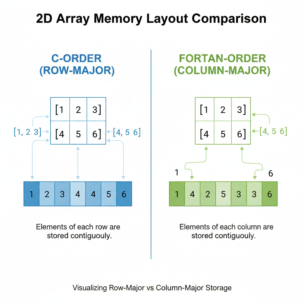 Row-major (C-order) stores rows contiguously — fast for row operations. Column-major (Fortran-order) stores columns contiguously — fast for column operations.
Understanding Strides
NumPy uses strides to navigate arrays without copying data:
arr = np.arange(12).reshape(3, 4)
print(arr)
# [[ 0  1  2  3]
#  [ 4  5  6  7]
#  [ 8  9 10 11]]

print(f"Shape: {arr.shape}")      # (3, 4)
print(f"Strides: {arr.strides}")  # (32, 8)
The strides (32, 8) mean:
- To move one row down: jump 32 bytes (4 elements × 8 bytes)
- To move one column right: jump 8 bytes (1 element × 8 bytes)
This is how NumPy can do transpose without copying:
arr_T = arr.T
print(f"Transposed strides: {arr_T.strides}")  # (8, 32) — just swapped!
print(f"Shares memory: {np.shares_memory(arr, arr_T)}")  # True
The transpose is just a different “view” of the same data — no copying, instant operation. This is a paradigm shift from Java where transpose() would create a whole new 2D array.
Vectorization: The BLAS/LAPACK Secret
Now we get to the real magic. When you write:
c = a + b # where a and b are NumPy arraysYou might think Python is doing something like:
c = np.empty_like(a)
for i in range(len(a)):
    c[i] = a[i] + b[i]
Wrong. What actually happens:
- NumPy checks the dtypes and shapes
- NumPy calls a compiled C function that:
- Uses SIMD instructions (SSE, AVX) to process 4-8 elements per CPU cycle
- Optionally uses multiple CPU cores (for large arrays)
- Uses BLAS/LAPACK for linear algebra operations
BLAS (Basic Linear Algebra Subprograms) and LAPACK are Fortran libraries from the 1970s-1990s that have been optimized by generations of performance engineers. They’re so good that even modern libraries use them.
Analogy for Android devs: This is like Android’s RenderThread offloading UI drawing to the GPU. Your main thread says “draw this list” and the RenderThread handles the optimized execution with GPU shaders. NumPy says “add these arrays” and BLAS handles the optimized execution with SIMD instructions.
 SIMD (Single Instruction, Multiple Data) processes 4-8 elements per CPU cycle. Instead of adding numbers one by one, the CPU adds entire vectors in parallel.
The Python Overhead Problem
The issue with Python loops isn’t that Python is slow — it’s that there’s overhead per operation:
# Python loop: overhead × N times
for i in range(1_000_000):
    c[i] = a[i] + b[i]
    # Each iteration:
    # - Python interprets the bytecode
    # - Fetches a[i] (dict lookup, bounds check)
    # - Fetches b[i] (dict lookup, bounds check)
    # - Adds them (type check, dispatch to __add__)
    # - Stores in c[i] (dict lookup, bounds check)
# NumPy: overhead once, then pure C
c = a + b
# Once:
# - Python calls np.add(a, b)
# - NumPy validates shapes and dtypes
# Then in C (no Python overhead):
# - SIMD loop processes millions of elementsThe Python overhead might be 100 nanoseconds. Do that 1 million times and you’ve added 100 milliseconds. NumPy pays that overhead once.
Broadcasting Rules: The Tricky Parts
Broadcasting is how NumPy handles operations between arrays of different shapes. It’s powerful but can be confusing.
The Basic Rule
When operating on two arrays, NumPy compares shapes from right to left. Dimensions are compatible if:
- They’re equal, OR
- One of them is 1
# Example 1: scalar + array (always works)
arr = np.array([1, 2, 3])
result = arr + 10  # 10 broadcasts to [10, 10, 10]
# Result: [11, 12, 13]

# Example 2: (3,) + (3, 3) — 1D broadcasts to rows
arr_1d = np.array([1, 2, 3])
arr_2d = np.array([[10, 20, 30],
                   [40, 50, 60],
                   [70, 80, 90]])
result = arr_1d + arr_2d
# arr_1d becomes [[1, 2, 3], [1, 2, 3], [1, 2, 3]]
# Result: [[11, 22, 33], [41, 52, 63], [71, 82, 93]]
The Edge Cases That Confuse People
# Case 1: (3, 1) + (1, 4) → (3, 4)
a = np.array([[1], [2], [3]])  # shape (3, 1)
b = np.array([[10, 20, 30, 40]])  # shape (1, 4)
result = a + b
# a broadcasts to:    [[1,  1,  1,  1],
#                      [2,  2,  2,  2],
#                      [3,  3,  3,  3]]
# b broadcasts to:    [[10, 20, 30, 40],
#                      [10, 20, 30, 40],
#                      [10, 20, 30, 40]]
print(result.shape)  # (3, 4)
# Case 2: (3,) + (4,) → ERROR
a = np.array([1, 2, 3]) # shape (3,)
b = np.array([1, 2, 3, 4]) # shape (4,)
# result = a + b # ValueError: shapes not aligned!# Case 3: (3, 4) + (4,) → (3, 4) — trailing dimension matches
a = np.array([[1, 2, 3, 4],
[5, 6, 7, 8],
[9, 10, 11, 12]]) # shape (3, 4)
b = np.array([10, 20, 30, 40]) # shape (4,)
result = a + b # b broadcasts to each row
# Result: [[11, 22, 33, 44], ...]My mental model: Think of it like CSS flexbox alignment. The dimensions stretch to fill the larger shape, but only if the smaller dimension is 1 or they match exactly.
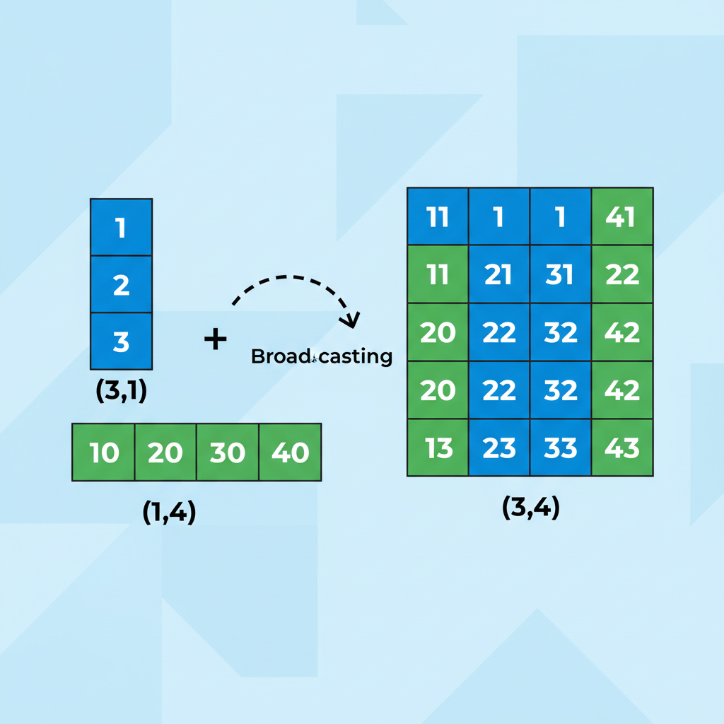 Broadcasting stretches dimensions to match. The (3,1) array expands horizontally, the (1,4) array expands vertically, producing a (3,4) result without copying data.
Views vs Copies: The Subtle Bugs
This is where I got bitten hard. Let me show you:
arr = np.array([1, 2, 3, 4, 5])

# This creates a VIEW (shares memory)
slice_view = arr[1:4]
slice_view[0] = 999

print(arr)  # [1, 999, 3, 4, 5] — ORIGINAL CHANGED!
Coming from Java, where Arrays.copyOfRange() always creates a new array, this was deeply unsettling. In NumPy, slicing creates a view — a new ndarray object that points to the same underlying data.
When It’s a View vs Copy
Views (shared memory):
- Basic slicing:
arr[1:4],arr[::2],arr[:, 0] - Transpose:
arr.T - Reshape (when possible):
arr.reshape(3, 4) - Ravel (when contiguous):
arr.ravel()
Copies (new memory):
- Fancy indexing:
arr[[1, 3, 4]],arr[arr > 2] - Explicit copy:
arr.copy() - Most operations:
arr + 1,np.sin(arr),arr * 2
How to Check
arr = np.arange(10)
slice_a = arr[2:5]      # View
slice_b = arr[[2, 3, 4]]  # Copy

print(np.shares_memory(arr, slice_a))  # True
print(np.shares_memory(arr, slice_b))  # False
The Safe Pattern
If you’re coming from Java and want predictable behavior, always copy when in doubt:
# Safe pattern: explicit copy
slice_safe = arr[1:4].copy()
slice_safe[0] = 999
print(arr)  # Original unchanged
Analogy for Android devs: This is like MutableLiveData vs LiveData. If you expose a MutableLiveData to the View layer, they can modify your state unexpectedly. NumPy views have the same danger — mutations propagate to the original array. Use .copy() like you’d use .asLiveData() to prevent unintended mutations.
The Benchmark: 4 Ways to Multiply Matrices
Let’s see the performance difference in action. We’ll multiply two 1000x1000 matrices:
import numpy as np
import time

n = 1000
A = np.random.rand(n, n)
B = np.random.rand(n, n)

# Method 1: Python nested loops (slowest)
def python_matmul(A, B):
    n = len(A)
    C = [[0.0] * n for _ in range(n)]
    for i in range(n):
        for j in range(n):
            for k in range(n):
                C[i][j] += A[i][k] * B[k][j]
    return C

# Method 2: NumPy with Python loop (still slow)
def numpy_loop_matmul(A, B):
    n = A.shape[0]
    C = np.zeros((n, n))
    for i in range(n):
        for j in range(n):
            C[i, j] = np.dot(A[i, :], B[:, j])
    return C

# Method 3: NumPy @ operator (fast)
def numpy_matmul(A, B):
    return A @ B

# Method 4: np.einsum (flexible and fast)
def einsum_matmul(A, B):
    return np.einsum('ik,kj->ij', A, B)

# Let's time them (only doing a subset for method 1 & 2)
print("Method 1 (Python loops, 100x100):")
A_small = np.random.rand(100, 100).tolist()
B_small = np.random.rand(100, 100).tolist()
start = time.time()
_ = python_matmul(A_small, B_small)
print(f"  Time: {time.time() - start:.3f}s")

print("\nMethod 2 (NumPy with loop, 100x100):")
A_small = np.random.rand(100, 100)
B_small = np.random.rand(100, 100)
start = time.time()
_ = numpy_loop_matmul(A_small, B_small)
print(f"  Time: {time.time() - start:.3f}s")

print("\nMethod 3 (NumPy @, 1000x1000):")
start = time.time()
_ = A @ B
print(f"  Time: {time.time() - start:.3f}s")

print("\nMethod 4 (einsum, 1000x1000):")
start = time.time()
_ = np.einsum('ik,kj->ij', A, B)
print(f"  Time: {time.time() - start:.3f}s")
Typical results on my MacBook:
Method 1 (Python loops, 100x100):
  Time: 1.247s

Method 2 (NumPy with loop, 100x100):
  Time: 0.089s

Method 3 (NumPy @, 1000x1000):
  Time: 0.021s

Method 4 (einsum, 1000x1000):
  Time: 0.058s
Method 1 takes 1.2 seconds for 100×100 matrices. Extrapolating to 1000×1000 (1000x more work): that’s ~1200 seconds = 20 minutes.
Method 3 does 1000×1000 in 0.02 seconds.
That’s a 60,000x speedup. Not a typo.
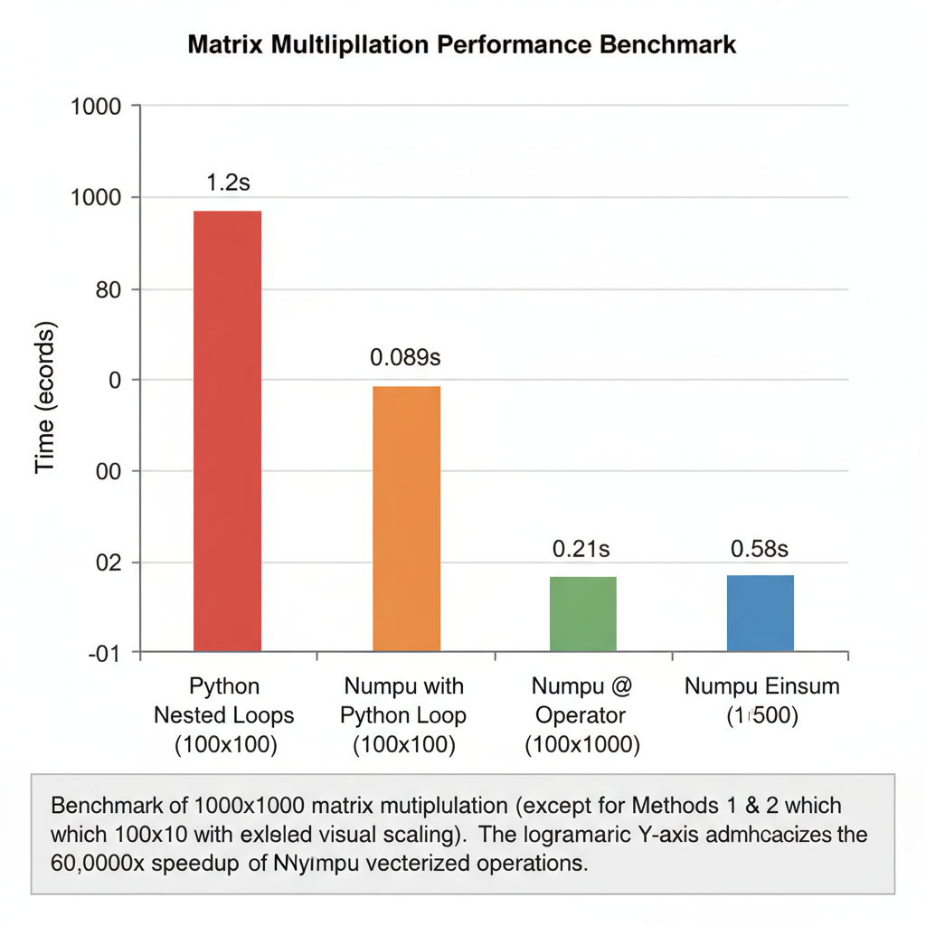 Python loops: 20 minutes. NumPy @: 0.02 seconds. The difference isn’t incremental — it’s transformational.
The Mental Model Shift
Here’s the paradigm change I wish someone had told me on day one:
Old thinking (imperative, from Java):
“Loop through each element and apply the operation.”
New thinking (declarative, NumPy):
“Describe the transformation you want on the whole array.”
It’s the same shift as going from:
// Imperative Java
List<Integer> doubled = new ArrayList<>();
for (int x : numbers) {
    doubled.add(x * 2);
}
To:
# Declarative NumPy
doubled = numbers * 2  # No loop in your code
Or think of SQL: you don’t write for each row in table: if row.age > 21: add to results. You write SELECT * FROM users WHERE age > 21. You describe the result, not the steps.
NumPy (and later pandas) work the same way. Stop thinking “iterate through elements.” Start thinking “describe the transformation.”
Practical Takeaways
When to Use NumPy vs Plain Python
Use NumPy when:
- Working with numerical data (arrays of numbers)
- Doing mathematical operations on collections
- Performance matters (data > 1000 elements)
- You need linear algebra operations
- Processing images, signals, or scientific data
Use plain Python when:
- Working with mixed types or complex objects
- The data is naturally nested/hierarchical (use dicts/classes)
- You’re doing string processing (use built-in str methods)
- The operations are inherently sequential with dependencies
The One Rule
Never loop over NumPy array elements in Python.
If you find yourself writing for i in range(len(arr)), stop. There’s almost always a vectorized way.
# BAD: Python loop
result = []
for x in arr:
    if x > threshold:
        result.append(x * 2)

# GOOD: Vectorized
mask = arr > threshold
result = arr[mask] * 2
Quick Reference: Common Operations
| Java/Python Loop | NumPy Vectorized |
|---|---|
for x in arr: total += x | arr.sum() |
max_val = max(arr) | arr.max() |
for i, x in enumerate(arr): arr[i] = x * 2 | arr *= 2 |
for i in range(len(a)): c[i] = a[i] + b[i] | c = a + b |
[x for x in arr if x > 0] | arr[arr > 0] |
[f(x) for x in arr] | np.vectorize(f)(arr) or better: find a NumPy function |
What’s Next
Tomorrow we tackle pandas — where the same vectorization principles apply, but for tabular data with labels, missing values, and mixed types. If NumPy is the foundation, pandas is the building.
The mental model: “Think in Transformations, Not Loops” will carry directly over. But pandas adds complexity: index alignment, the dreaded SettingWithCopyWarning, and the question of when to use pandas vs when it becomes the bottleneck.
Coming from a world where Room/SQLite handles our relational data needs, pandas is going to feel both familiar (it’s like SQL) and foreign (it’s mutable and full of gotchas).
See you in Day 3.
Resources for going deeper:
- NumPy Internals Documentation
- From Python to NumPy by Nicolas P. Rougier
- NumPy Broadcasting