Pandas for Data Manipulation: An Android Developer's Guide
In the last post, we dove deep into NumPy and discovered why vectorization gives us 60,000x speedups over naive Python loops. Today, we’re building on that foundation with pandas — the library that turns raw data into insights.
If NumPy is like Android’s ByteBuffer (low-level, fast, precise), then pandas is like Room with LiveData — higher-level abstractions that handle the messy reality of real-world data while still being performant under the hood.
Let’s dive in.
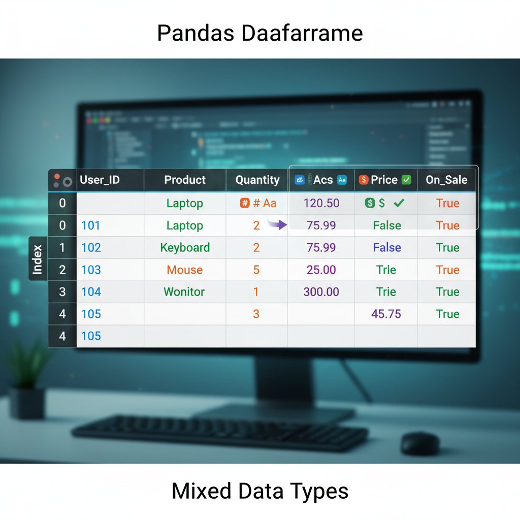 Diagram: A DataFrame visualized as a spreadsheet-like table with labeled rows (index) and columns, showing how data is organized in a 2D structure with mixed data types.
Why Pandas? The 10-Second Pitch
Here’s the reality of data science work: 80% of your time is spent cleaning and preparing data. Not training models. Not tuning hyperparameters. Just wrestling with missing values, inconsistent formats, and joining datasets that don’t quite match up.
Pandas is the tool that makes that 80% bearable.
import pandas as pd

# Load a CSV, handle missing values, filter, group, and aggregate
# All in one readable chain
df = (pd.read_csv('sales.csv')
      .dropna(subset=['revenue'])
      .query('region == "APAC"')
      .groupby('product')
      .agg({'revenue': 'sum', 'units': 'mean'})
      .sort_values('revenue', ascending=False))
That’s six operations that would take 50+ lines in Java. And it runs on NumPy under the hood, so it’s fast.
The Mental Model: DataFrame as RecyclerView.Adapter
Here’s the analogy that made pandas click for me as an Android developer.
A DataFrame is like a RecyclerView.Adapter backed by a database table:
| Pandas Concept | Android Equivalent |
|---|---|
DataFrame | RecyclerView.Adapter + data source |
Series (single column) | List<T> for one field |
Index | Primary key / @PrimaryKey |
df.loc[] | getItemAt(position) |
df.query() | Room’s @Query with WHERE clause |
df.groupby() | SQL GROUP BY in Room |
df.merge() | Room @Relation / JOIN |
But unlike RecyclerView.Adapter, pandas lets you transform the entire dataset in one operation without writing loops. It’s declarative, not imperative.
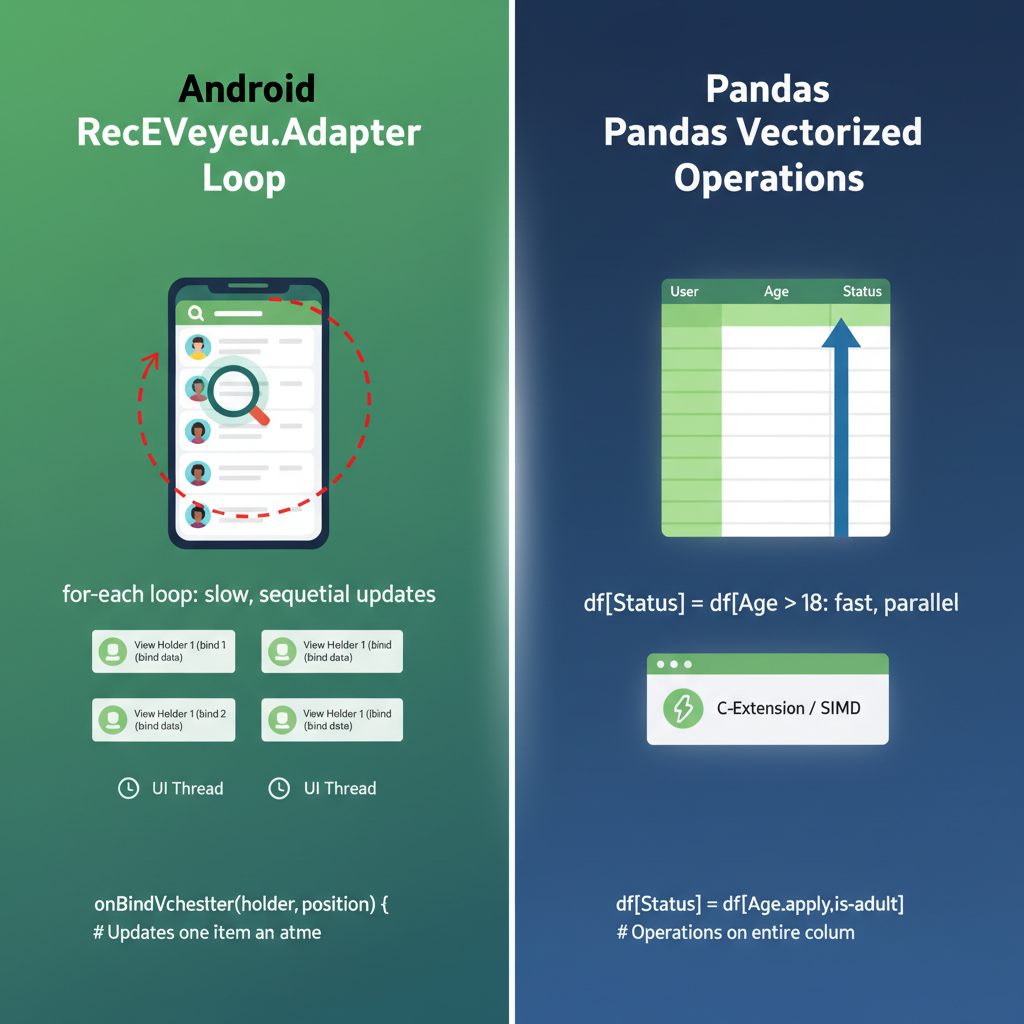 Diagram: Side-by-side comparison showing Android RecyclerView.Adapter architecture (ViewHolder, onBindViewHolder loop) vs pandas DataFrame operations (vectorized transformations). Highlight the “loop vs no-loop” difference.
Series: The Building Block
A Series is a 1D labeled array. Think of it as a Map<Index, Value> that maintains insertion order and supports vectorized operations.
import pandas as pd

# Creating a Series
revenue = pd.Series([1000, 2500, 1800, 3200],
                    index=['Q1', 'Q2', 'Q3', 'Q4'],
                    name='revenue')

print(revenue)
# Q1    1000
# Q2    2500
# Q3    1800
# Q4    3200
# Name: revenue, dtype: int64
Vectorized Operations on Series
Remember from the NumPy post — no loops needed:
# Apply 10% growth to all quarters
revenue_with_growth = revenue * 1.10

# Boolean indexing (like a filter)
high_performers = revenue[revenue > 2000]
# Q2    2500
# Q4    3200

# Apply functions
revenue.apply(lambda x: 'High' if x > 2000 else 'Low')
# Q1     Low
# Q2    High
# Q3     Low
# Q4    High
In Java, that last operation would be:
List<String> categories = new ArrayList<>();
for (Integer r : revenues) {
    categories.add(r > 2000 ? "High" : "Low");
}
Pandas does it in one line, and it’s faster because it’s running on NumPy arrays underneath.
DataFrame: The Star of the Show
A DataFrame is a 2D table — essentially a dictionary of Series objects sharing the same index.
# Creating a DataFrame
data = {
    'product': ['App A', 'App B', 'App C', 'App D'],
    'downloads': [50000, 120000, 30000, 85000],
    'revenue': [5000, 15000, 2000, 12000],
    'rating': [4.5, 4.8, 3.9, 4.2]
}

df = pd.DataFrame(data)
print(df)
#   product  downloads  revenue  rating
# 0   App A      50000     5000     4.5
# 1   App B     120000    15000     4.8
# 2   App C      30000     2000     3.9
# 3   App D      85000    12000     4.2
Reading Real Data
In practice, you rarely create DataFrames manually. You load them from files:
# CSV (most common)
df = pd.read_csv('data.csv')

# Excel
df = pd.read_excel('data.xlsx', sheet_name='Sheet1')

# JSON (familiar from Android Retrofit!)
df = pd.read_json('data.json')

# SQL database
import sqlite3
conn = sqlite3.connect('app.db')
df = pd.read_sql('SELECT * FROM users', conn)
That last one is particularly satisfying for Android developers. Same SQL, different runtime.
Selecting Data: .loc vs .iloc
This is where pandas gets confusing for beginners. There are two primary ways to select data:
.loc[]— Label-based selection (like HashMap lookup by key).iloc[]— Integer-based selection (like ArrayList index)
df = pd.DataFrame({
    'name': ['Alice', 'Bob', 'Charlie'],
    'score': [85, 92, 78]
}, index=['a', 'b', 'c'])  # Custom string index

# .loc uses labels
df.loc['a']           # Row with index 'a'
df.loc['a', 'score']  # Single value: 85
df.loc['a':'b']       # Rows 'a' through 'b' (inclusive!)

# .iloc uses integer positions
df.iloc[0]            # First row (same as df.loc['a'])
df.iloc[0, 1]         # First row, second column: 85
df.iloc[0:2]          # First two rows (exclusive end, like Python)
The gotcha: .loc[] slicing is inclusive on both ends. .iloc[] slicing is exclusive on the end, like normal Python slicing.
As an Android developer, I think of it this way:
.iloc[]is likelist.subList(0, 2)— exclusive end.loc[]is like SQL’sBETWEEN— inclusive on both ends
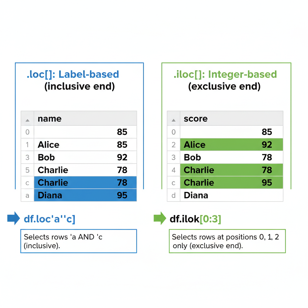 Diagram: A DataFrame with both integer positions (0, 1, 2) and string labels (‘a’, ‘b’, ‘c’) as index. Show how .loc[‘a’:‘b’] selects rows ‘a’ AND ‘b’ (inclusive), while .iloc[0:2] selects positions 0 and 1 only (exclusive end). Use color highlighting to show selected vs excluded rows.
Filtering: The Query Method
Here’s where pandas feels like writing Room queries:
# SQL: SELECT * FROM df WHERE downloads > 50000 AND rating >= 4.0
filtered = df.query('downloads > 50000 and rating >= 4.0')

# Or with boolean indexing (more explicit)
filtered = df[(df['downloads'] > 50000) & (df['rating'] >= 4.0)]
Note the & instead of and in boolean indexing. This trips up everyone at first. The parentheses are also required due to operator precedence.
I prefer .query() for complex conditions — it reads like SQL and doesn’t require the parentheses dance.
Dynamic Queries with Variables
min_downloads = 50000
min_rating = 4.0

# Use @ to reference Python variables in query strings
filtered = df.query('downloads > @min_downloads and rating >= @min_rating')
This feels just like parameterized queries in Room. The @ prefix tells pandas to look up the variable in the local scope.
Handling Missing Data: The NaN Reality
In Android, null handling is explicit — @Nullable, Optional<T>, null checks. In pandas, missing data is represented as NaN (Not a Number), and it propagates silently through operations if you’re not careful.
import numpy as np

df = pd.DataFrame({
    'name': ['Alice', 'Bob', 'Charlie', 'Diana'],
    'score': [85, np.nan, 78, 92],
    'grade': ['A', 'B', None, 'A']
})

# Check for missing values
df.isna()
#     name  score  grade
# 0  False  False  False
# 1  False   True  False
# 2  False  False   True
# 3  False  False  False

# Count missing values per column
df.isna().sum()
# name     0
# score    1
# grade    1

# Drop rows with any NaN
df_clean = df.dropna()

# Fill NaN with a value
df_filled = df.fillna({'score': 0, 'grade': 'Unknown'})

# Forward fill (use previous value)
df['score'].ffill()
The isna() vs isnull() Confusion
They’re identical. isnull() is an alias for isna(). Pick one and stick with it. I use isna() because it’s more explicit.
GroupBy: SQL-Style Aggregation
This is one of pandas’ superpowers. It’s like combining SQL’s GROUP BY with Java Streams’ Collectors.groupingBy().
# Sample data: app usage by region
usage = pd.DataFrame({
    'region': ['APAC', 'APAC', 'NA', 'NA', 'EU', 'EU'],
    'product': ['App A', 'App B', 'App A', 'App B', 'App A', 'App B'],
    'users': [5000, 8000, 12000, 15000, 7000, 9000],
    'revenue': [50000, 80000, 120000, 150000, 70000, 90000]
})

# Group by region, sum the numeric columns
by_region = usage.groupby('region').sum()
#        users  revenue
# region
# APAC   13000   130000
# EU     16000   160000
# NA     27000   270000

# Multiple aggregations
by_region = usage.groupby('region').agg({
    'users': 'sum',
    'revenue': ['sum', 'mean']
})

# Group by multiple columns
by_region_product = usage.groupby(['region', 'product']).sum()
The Split-Apply-Combine Pattern
Under the hood, groupby() follows the split-apply-combine pattern:
- Split: Divide the DataFrame into groups based on key(s)
- Apply: Apply a function to each group independently
- Combine: Merge the results back into a DataFrame
This is exactly how I think about RecyclerView’s ItemDecoration with section headers — you split items by category, apply formatting to each section, and combine them into the final list.
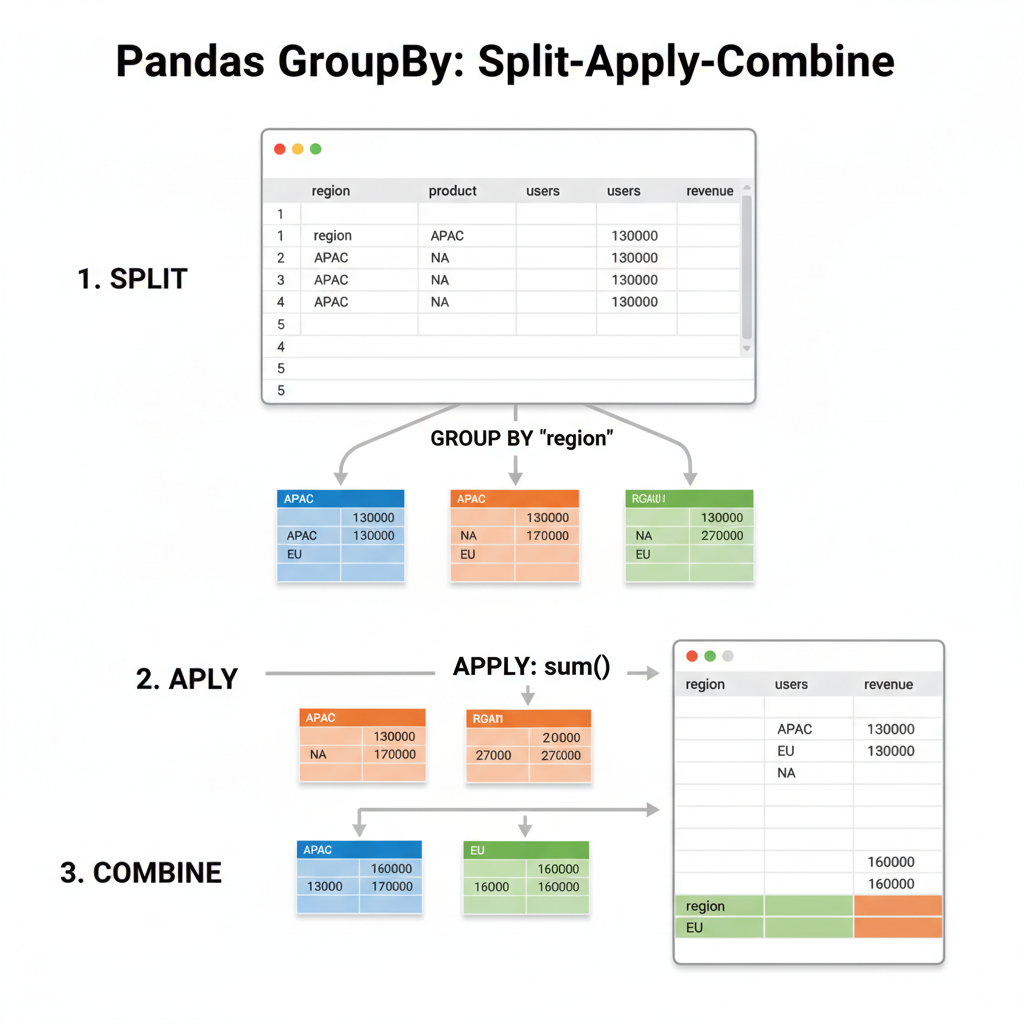 Diagram: Three-step visualization showing: (1) SPLIT - a DataFrame being divided into colored groups by region (APAC=blue, EU=green, NA=orange), (2) APPLY - each group having sum() applied independently, (3) COMBINE - results merged back into a single summary DataFrame. Use arrows to show the flow.
# Custom aggregation with apply
def revenue_per_user(group):
    return pd.Series({
        'total_users': group['users'].sum(),
        'total_revenue': group['revenue'].sum(),
        'arpu': group['revenue'].sum() / group['users'].sum()
    })

usage.groupby('region').apply(revenue_per_user)
Merging DataFrames: The JOIN Equivalent
If you’ve written Room relations with @Embedded and @Relation, you’ll feel right at home with pandas merge operations.
# Two tables to join
users = pd.DataFrame({
    'user_id': [1, 2, 3, 4],
    'name': ['Alice', 'Bob', 'Charlie', 'Diana']
})

orders = pd.DataFrame({
    'order_id': [101, 102, 103, 104, 105],
    'user_id': [1, 2, 1, 3, 5],  # Note: user 5 doesn't exist in users
    'amount': [50, 75, 30, 100, 25]
})

# Inner join (default) - only matching records
merged = pd.merge(users, orders, on='user_id')
# user_id     name  order_id  amount
#       1    Alice       101      50
#       1    Alice       103      30
#       2      Bob       102      75
#       3  Charlie       104     100

# Left join - all users, matched orders or NaN
merged = pd.merge(users, orders, on='user_id', how='left')

# Outer join - all records from both tables
merged = pd.merge(users, orders, on='user_id', how='outer')
Pandas how= | SQL Equivalent | Room Equivalent |
|---|---|---|
'inner' | INNER JOIN | @Relation with matching keys |
'left' | LEFT OUTER JOIN | @Relation with nullable result |
'right' | RIGHT OUTER JOIN | (less common) |
'outer' | FULL OUTER JOIN | (manual implementation) |
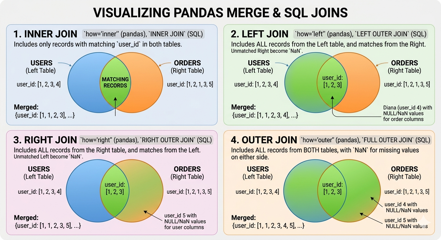 Diagram: Four Venn diagram-style illustrations showing INNER (intersection only), LEFT (all left + matching right), RIGHT (all right + matching left), and OUTER (union of both) joins. Use two overlapping circles representing ‘users’ and ‘orders’ tables, with colored regions showing which records are included in each join type.
Method Chaining: Pandas’ Fluent API
One of the things I love about Kotlin is method chaining with scope functions. Pandas has a similar fluent API that makes data pipelines readable:
# The ugly way (intermediate variables)
df1 = pd.read_csv('sales.csv')
df2 = df1.dropna()
df3 = df2[df2['region'] == 'APAC']
df4 = df3.groupby('product').sum()
result = df4.sort_values('revenue', ascending=False)

# The pandas way (method chaining)
result = (pd.read_csv('sales.csv')
          .dropna()
          .query('region == "APAC"')
          .groupby('product')
          .sum()
          .sort_values('revenue', ascending=False))
The parentheses allow line breaks without backslashes. This reads almost like a SQL query or a Kotlin Flow chain.
The .pipe() Method for Custom Functions
When you need to insert custom logic into a chain:
def add_revenue_category(df):
    df['category'] = pd.cut(df['revenue'],
                           bins=[0, 1000, 10000, float('inf')],
                           labels=['Small', 'Medium', 'Large'])
    return df

result = (pd.read_csv('sales.csv')
          .dropna()
          .pipe(add_revenue_category)  # Custom function in the chain
          .groupby('category')
          .sum())
This is like Kotlin’s .let{} — it lets you inject arbitrary transformations into a fluent chain.
Performance Considerations
The Vectorization Rule Still Applies
Everything we learned about NumPy vectorization applies to pandas:
import numpy as np

# SLOW: iterating over rows
def slow_calculate(df):
    results = []
    for idx, row in df.iterrows():
        results.append(row['a'] * 2 + row['b'])
    return results

# FAST: vectorized operation
def fast_calculate(df):
    return df['a'] * 2 + df['b']
Benchmark on 1 million rows:
iterrows()version: ~45 seconds- Vectorized version: ~15 milliseconds
That’s a 3000x speedup. Never use iterrows() for computation.
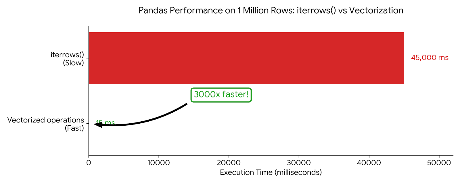 Chart: Horizontal bar chart comparing iterrows() (45,000ms, red/slow) vs vectorized operations (15ms, green/fast) on 1 million rows. Include a “3000x faster” callout. The visual scale should make the dramatic difference obvious.
Memory Efficiency with dtypes
Pandas infers dtypes when reading data, but it’s often wasteful:
df = pd.read_csv('users.csv')
df.dtypes
# user_id      int64     # 8 bytes per value
# age          int64     # 8 bytes, but ages fit in int8!
# is_premium   object    # Python objects, very expensive

# Optimize
df['age'] = df['age'].astype('int8')           # 1 byte
df['is_premium'] = df['is_premium'].astype('bool')  # 1 byte (was ~50+ bytes)
df['user_id'] = df['user_id'].astype('int32')  # 4 bytes

# Or specify dtypes on read
df = pd.read_csv('users.csv', dtype={
    'user_id': 'int32',
    'age': 'int8',
    'is_premium': 'bool'
})
This is just like choosing the right data types in Android to minimize APK size and memory footprint.
The Category dtype for Strings
If a string column has repeated values (like regions, categories, status), use category:
# Before: each 'APAC' string is stored separately
df['region'].memory_usage(deep=True)  # 800000 bytes

# After: integers with a lookup table
df['region'] = df['region'].astype('category')
df['region'].memory_usage(deep=True)  # 100300 bytes (88% reduction!)
This is exactly like Android’s string resources — store once, reference many times.
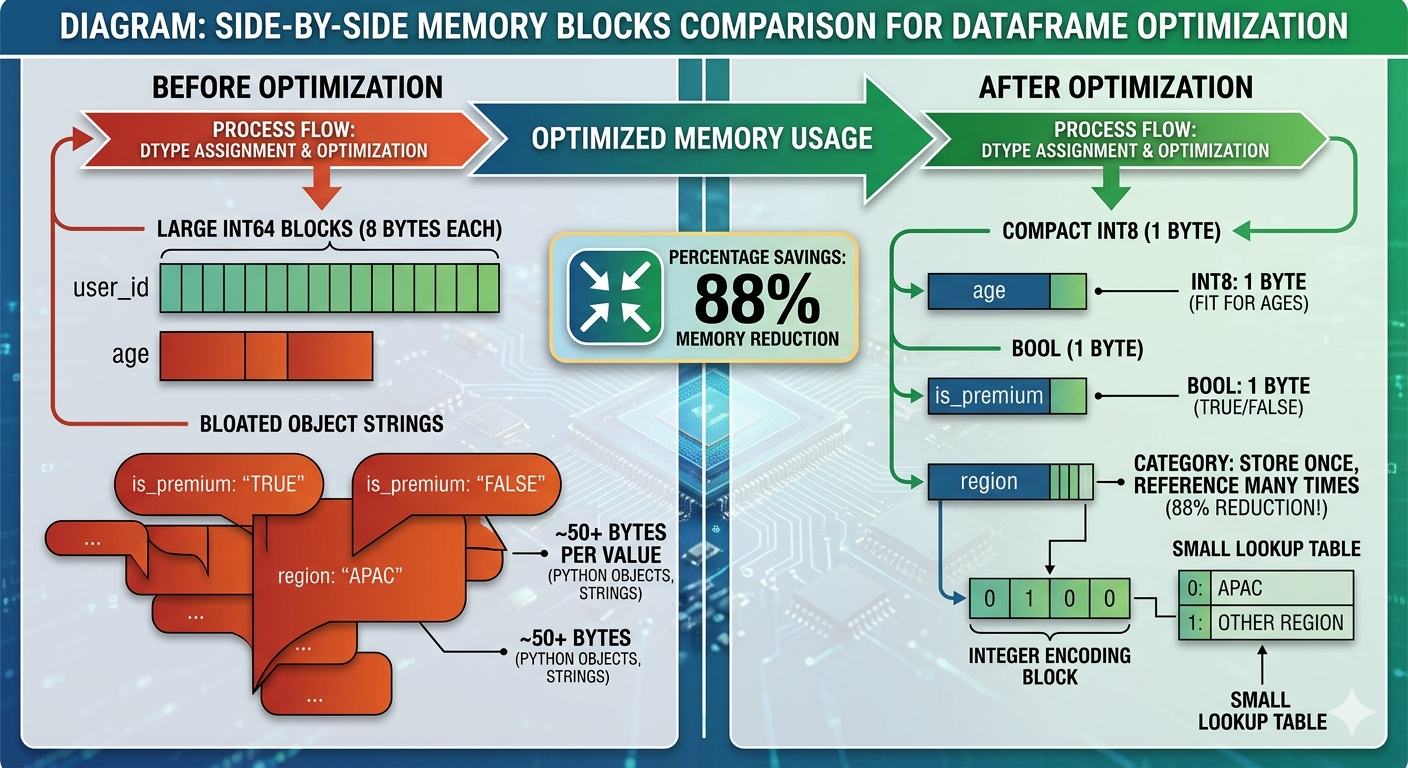 Diagram: Side-by-side memory blocks comparison. Left side shows “Before optimization” with large int64 blocks (8 bytes each) and bloated object strings. Right side shows “After optimization” with compact int8 (1 byte), bool (1 byte), and category dtype (integer + small lookup table). Include percentage savings: “88% memory reduction”.
Common Gotchas
1. The SettingWithCopyWarning
This is the most confusing error for pandas beginners:
# This might work, but is it a view or a copy?
subset = df[df['score'] > 80]
subset['grade'] = 'A'  # SettingWithCopyWarning!
The issue: df[df['score'] > 80] might return a view (shared memory) or a copy (independent memory). Modifying it could affect the original df… or not.
The fix: Be explicit about copies:
# Explicit copy
subset = df[df['score'] > 80].copy()
subset['grade'] = 'A'  # Safe, no warning

# Or use .loc for in-place modification of original
df.loc[df['score'] > 80, 'grade'] = 'A'  # Modifies df directly
2. Chained Indexing is Evil
# BAD: chained indexing (unpredictable)
df['score'][0] = 100

# GOOD: single .loc call
df.loc[0, 'score'] = 100
3. The Index Alignment “Feature”
When operating on two Series, pandas aligns by index, not position:
s1 = pd.Series([1, 2, 3], index=['a', 'b', 'c'])
s2 = pd.Series([10, 20, 30], index=['b', 'c', 'd'])

s1 + s2
# a     NaN  # No 'a' in s2
# b    12.0  # 2 + 10
# c    23.0  # 3 + 20
# d     NaN  # No 'd' in s1
This is powerful for time series data, but surprising if you expect position-based operations. Use .values to get raw NumPy arrays if you need position-based math.
Practical Example: Analyzing App Store Data
Let’s put it all together with a realistic example — analyzing app download data:
import pandas as pd
import numpy as np

# Load data
df = pd.read_csv('app_downloads.csv')

# Initial exploration
print(df.shape)           # (rows, columns)
print(df.dtypes)          # Column types
print(df.describe())      # Statistical summary
print(df.isna().sum())    # Missing values per column

# Clean the data
df_clean = (df
    .dropna(subset=['revenue', 'downloads'])  # Required fields
    .fillna({'rating': df['rating'].median()})  # Fill optional with median
    .query('downloads > 0')  # Remove invalid records
)

# Feature engineering
df_clean['revenue_per_download'] = df_clean['revenue'] / df_clean['downloads']
df_clean['is_high_rated'] = df_clean['rating'] >= 4.5

# Analyze by category
summary = (df_clean
    .groupby('category')
    .agg({
        'downloads': ['sum', 'mean'],
        'revenue': ['sum', 'mean'],
        'revenue_per_download': 'mean',
        'is_high_rated': 'mean'  # Proportion of high-rated apps
    })
    .round(2)
    .sort_values(('revenue', 'sum'), ascending=False)
)

print(summary)
This is the kind of analysis that would take hundreds of lines in Java, with manual null checks, loops, and temporary collections. Pandas does it in a few readable lines.
What’s Next
We’ve covered the core of pandas — enough to start doing real data analysis. In the next post, we’ll tackle data visualization with matplotlib and seaborn — turning these DataFrames into charts that tell a story.
But the real test comes when you apply these tools to messy, real-world data. The Kaggle dataset that looked clean in the preview? It has Unicode issues, mixed date formats, and columns that should be numbers but are stored as strings with commas.
That’s where the 80% of data science work happens. And now you have the tools to handle it.
Key Takeaways
- DataFrame = Table: Think of it as a dictionary of Series (columns) with a shared index
- Vectorize everything: Never use
iterrows()for computation .loc[]for labels,.iloc[]for positions: Remember the inclusive vs exclusive slicing difference- Method chaining: Write pipelines, not intermediate variables
- Be explicit about copies: Use
.copy()to avoid the SettingWithCopyWarning - Optimize dtypes: Use
categoryfor repeated strings, smaller ints for bounded values
For Android developers, the mental model shift is similar to going from imperative Java to declarative Kotlin Flow or Compose. You describe what you want, not how to compute it step by step.
See you in the next post!
Happy learning!