Pandas cho Xử lý Dữ liệu: Hướng dẫn dành cho Android Developer
Trong bài trước, chúng ta đã tìm hiểu sâu về NumPy và khám phá tại sao vectorization cho tốc độ nhanh hơn 60,000 lần so với loop Python thông thường. Hôm nay, chúng ta sẽ xây dựng tiếp trên nền tảng đó với pandas — thư viện biến dữ liệu thô thành insights.
Nếu NumPy giống như ByteBuffer của Android (low-level, nhanh, chính xác), thì pandas giống như Room với LiveData — abstraction cấp cao hơn, xử lý được sự phức tạp của dữ liệu thực tế mà vẫn performant bên dưới.
Bắt đầu thôi.
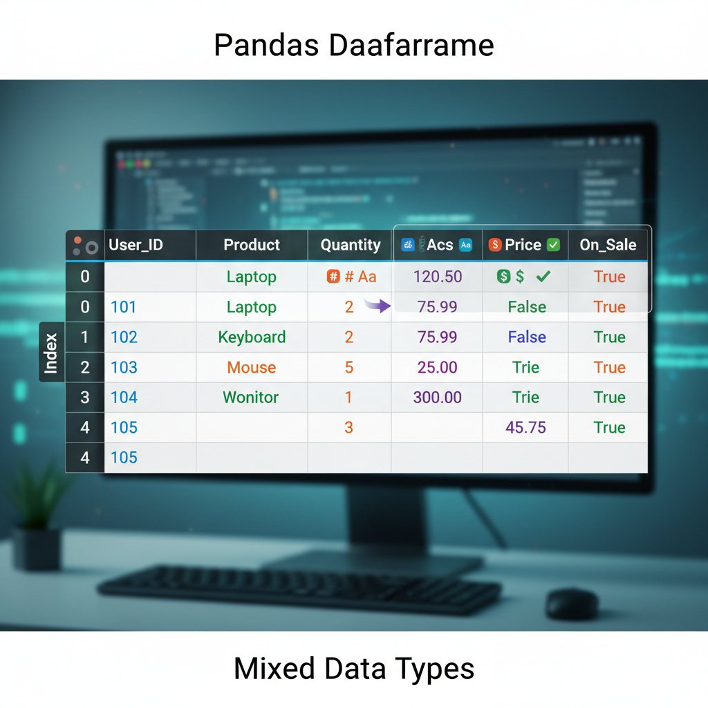 Sơ đồ: DataFrame được visualize như một bảng dạng spreadsheet với labeled rows (index) và columns, thể hiện cách dữ liệu được tổ chức trong cấu trúc 2D với nhiều data type khác nhau.
Tại sao Pandas? Pitch 10 giây
Đây là thực tế của công việc data science: 80% thời gian của bạn dành cho việc cleaning và chuẩn bị dữ liệu. Không phải training model. Không phải tuning hyperparameters. Chỉ là vật lộn với missing values, format không nhất quán, và join các dataset không khớp nhau.
Pandas là công cụ giúp 80% đó dễ chịu hơn.
import pandas as pd

# Load CSV, xử lý missing values, filter, group, và aggregate
# Tất cả trong một chain dễ đọc
df = (pd.read_csv('sales.csv')
      .dropna(subset=['revenue'])
      .query('region == "APAC"')
      .groupby('product')
      .agg({'revenue': 'sum', 'units': 'mean'})
      .sort_values('revenue', ascending=False))
Đó là 6 operations mà trong Java sẽ cần 50+ dòng code. Và nó chạy trên NumPy bên dưới, nên rất nhanh.
Mental Model: DataFrame như RecyclerView.Adapter
Đây là analogy giúp mình hiểu pandas với tư cách một Android developer.
Một DataFrame giống như một RecyclerView.Adapter được back bởi một database table:
| Khái niệm Pandas | Tương đương Android |
|---|---|
DataFrame | RecyclerView.Adapter + data source |
Series (single column) | List<T> cho một field |
Index | Primary key / @PrimaryKey |
df.loc[] | getItemAt(position) |
df.query() | Room’s @Query với WHERE clause |
df.groupby() | SQL GROUP BY trong Room |
df.merge() | Room @Relation / JOIN |
Nhưng khác với RecyclerView.Adapter, pandas cho phép bạn transform toàn bộ dataset trong một operation mà không cần viết loop. Nó là declarative, không phải imperative.
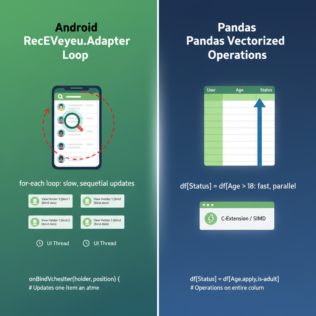 Sơ đồ: So sánh cạnh nhau giữa kiến trúc Android RecyclerView.Adapter (ViewHolder, vòng lặp onBindViewHolder) với pandas DataFrame operations (vectorized transformations). Highlight sự khác biệt “loop vs no-loop”.
Series: Khối xây dựng cơ bản
Một Series là labeled array 1D. Hãy nghĩ nó như một Map<Index, Value> giữ nguyên thứ tự insertion và hỗ trợ vectorized operations.
import pandas as pd

# Tạo một Series
revenue = pd.Series([1000, 2500, 1800, 3200],
                    index=['Q1', 'Q2', 'Q3', 'Q4'],
                    name='revenue')

print(revenue)
# Q1    1000
# Q2    2500
# Q3    1800
# Q4    3200
# Name: revenue, dtype: int64
Vectorized Operations trên Series
Nhớ từ bài NumPy — không cần loop:
# Áp dụng tăng trưởng 10% cho tất cả các quý
revenue_with_growth = revenue * 1.10

# Boolean indexing (giống filter)
high_performers = revenue[revenue > 2000]
# Q2    2500
# Q4    3200

# Apply functions
revenue.apply(lambda x: 'High' if x > 2000 else 'Low')
# Q1     Low
# Q2    High
# Q3     Low
# Q4    High
Trong Java, operation cuối sẽ là:
List<String> categories = new ArrayList<>();
for (Integer r : revenues) {
    categories.add(r > 2000 ? "High" : "Low");
}
Pandas làm trong một dòng, và nhanh hơn vì nó chạy trên NumPy arrays bên dưới.
DataFrame: Ngôi sao của show
Một DataFrame là bảng 2D — về cơ bản là một dictionary của các Series objects chia sẻ cùng index.
# Tạo một DataFrame
data = {
    'product': ['App A', 'App B', 'App C', 'App D'],
    'downloads': [50000, 120000, 30000, 85000],
    'revenue': [5000, 15000, 2000, 12000],
    'rating': [4.5, 4.8, 3.9, 4.2]
}

df = pd.DataFrame(data)
print(df)
#   product  downloads  revenue  rating
# 0   App A      50000     5000     4.5
# 1   App B     120000    15000     4.8
# 2   App C      30000     2000     3.9
# 3   App D      85000    12000     4.2
Đọc dữ liệu thực
Trong thực tế, hiếm khi bạn tạo DataFrame thủ công. Bạn load chúng từ files:
# CSV (phổ biến nhất)
df = pd.read_csv('data.csv')

# Excel
df = pd.read_excel('data.xlsx', sheet_name='Sheet1')

# JSON (quen thuộc với Android Retrofit!)
df = pd.read_json('data.json')

# SQL database
import sqlite3
conn = sqlite3.connect('app.db')
df = pd.read_sql('SELECT * FROM users', conn)
Cái cuối đặc biệt thỏa mãn với Android developers. Cùng SQL, khác runtime.
Chọn dữ liệu: .loc vs .iloc
Đây là chỗ pandas gây confused cho người mới. Có hai cách chính để select data:
.loc[]— Label-based selection (như HashMap lookup by key).iloc[]— Integer-based selection (như ArrayList index)
df = pd.DataFrame({
    'name': ['Alice', 'Bob', 'Charlie'],
    'score': [85, 92, 78]
}, index=['a', 'b', 'c'])  # Custom string index

# .loc dùng labels
df.loc['a']           # Row với index 'a'
df.loc['a', 'score']  # Single value: 85
df.loc['a':'b']       # Rows 'a' đến 'b' (inclusive!)

# .iloc dùng integer positions
df.iloc[0]            # Row đầu tiên (giống df.loc['a'])
df.iloc[0, 1]         # Row đầu tiên, column thứ hai: 85
df.iloc[0:2]          # Hai row đầu (exclusive end, như Python)
Cạm bẫy: .loc[] slicing là inclusive cả hai đầu. .iloc[] slicing là exclusive ở cuối, như Python slicing thông thường.
Với tư cách Android developer, mình nghĩ như thế này:
.iloc[]giốnglist.subList(0, 2)— exclusive end.loc[]giống SQL’sBETWEEN— inclusive cả hai đầu
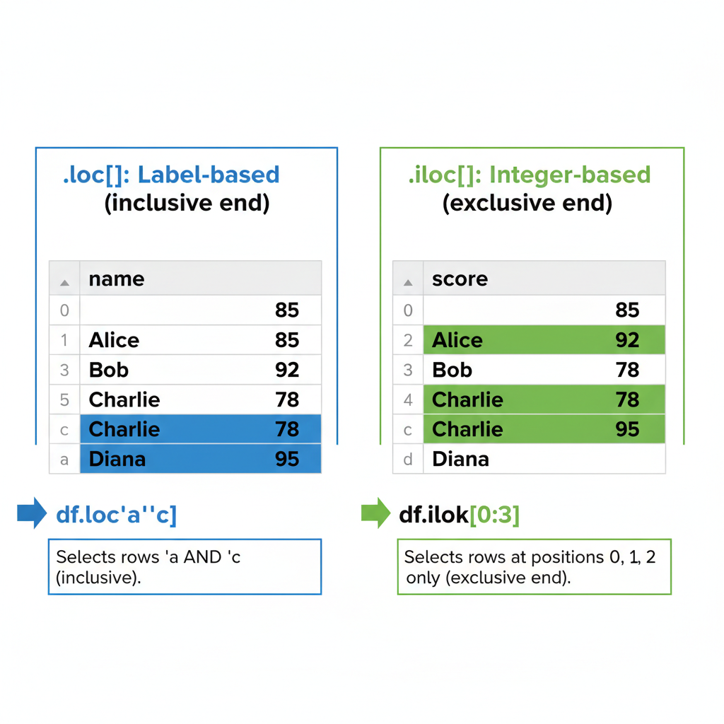 Sơ đồ: Một DataFrame với cả integer positions (0, 1, 2) và string labels (‘a’, ‘b’, ‘c’) làm index. Cho thấy .loc[‘a’:‘b’] chọn rows ‘a’ VÀ ‘b’ (inclusive), trong khi .iloc[0:2] chỉ chọn positions 0 và 1 (exclusive end). Dùng color highlighting để phân biệt selected vs excluded rows.
Filtering: Query Method
Đây là chỗ pandas cảm giác như viết Room queries:
# SQL: SELECT * FROM df WHERE downloads > 50000 AND rating >= 4.0
filtered = df.query('downloads > 50000 and rating >= 4.0')

# Hoặc với boolean indexing (explicit hơn)
filtered = df[(df['downloads'] > 50000) & (df['rating'] >= 4.0)]
Chú ý & thay vì and trong boolean indexing. Ai cũng bị lần đầu. Các dấu ngoặc cũng bắt buộc do operator precedence.
Mình prefer .query() cho các điều kiện phức tạp — nó đọc như SQL và không cần nhảy múa với dấu ngoặc.
Dynamic Queries với Variables
min_downloads = 50000
min_rating = 4.0

# Dùng @ để reference Python variables trong query strings
filtered = df.query('downloads > @min_downloads and rating >= @min_rating')
Cảm giác y như parameterized queries trong Room. Prefix @ nói với pandas tìm variable trong local scope.
Xử lý Missing Data: Thực tế NaN
Trong Android, null handling là explicit — @Nullable, Optional<T>, null checks. Trong pandas, missing data được biểu diễn là NaN (Not a Number), và nó lan truyền im lặng qua các operations nếu bạn không cẩn thận.
import numpy as np

df = pd.DataFrame({
    'name': ['Alice', 'Bob', 'Charlie', 'Diana'],
    'score': [85, np.nan, 78, 92],
    'grade': ['A', 'B', None, 'A']
})

# Check missing values
df.isna()
#     name  score  grade
# 0  False  False  False
# 1  False   True  False
# 2  False  False   True
# 3  False  False  False

# Đếm missing values mỗi column
df.isna().sum()
# name     0
# score    1
# grade    1

# Drop rows có NaN
df_clean = df.dropna()

# Fill NaN với một giá trị
df_filled = df.fillna({'score': 0, 'grade': 'Unknown'})

# Forward fill (dùng giá trị trước đó)
df['score'].ffill()
Sự nhầm lẫn isna() vs isnull()
Chúng giống hệt nhau. isnull() là alias của isna(). Chọn một cái và stick với nó. Mình dùng isna() vì nó explicit hơn.
GroupBy: Aggregation kiểu SQL
Đây là một trong những siêu năng lực của pandas. Giống như kết hợp SQL’s GROUP BY với Java Streams’ Collectors.groupingBy().
# Sample data: app usage theo region
usage = pd.DataFrame({
    'region': ['APAC', 'APAC', 'NA', 'NA', 'EU', 'EU'],
    'product': ['App A', 'App B', 'App A', 'App B', 'App A', 'App B'],
    'users': [5000, 8000, 12000, 15000, 7000, 9000],
    'revenue': [50000, 80000, 120000, 150000, 70000, 90000]
})

# Group by region, sum các numeric columns
by_region = usage.groupby('region').sum()
#        users  revenue
# region
# APAC   13000   130000
# EU     16000   160000
# NA     27000   270000

# Multiple aggregations
by_region = usage.groupby('region').agg({
    'users': 'sum',
    'revenue': ['sum', 'mean']
})

# Group by multiple columns
by_region_product = usage.groupby(['region', 'product']).sum()
Pattern Split-Apply-Combine
Bên dưới, groupby() theo pattern split-apply-combine:
- Split: Chia DataFrame thành các groups dựa trên key(s)
- Apply: Apply một function lên mỗi group độc lập
- Combine: Merge kết quả lại thành một DataFrame
Đây chính xác là cách mình nghĩ về RecyclerView’s ItemDecoration với section headers — bạn split items theo category, apply formatting cho mỗi section, và combine chúng thành final list.
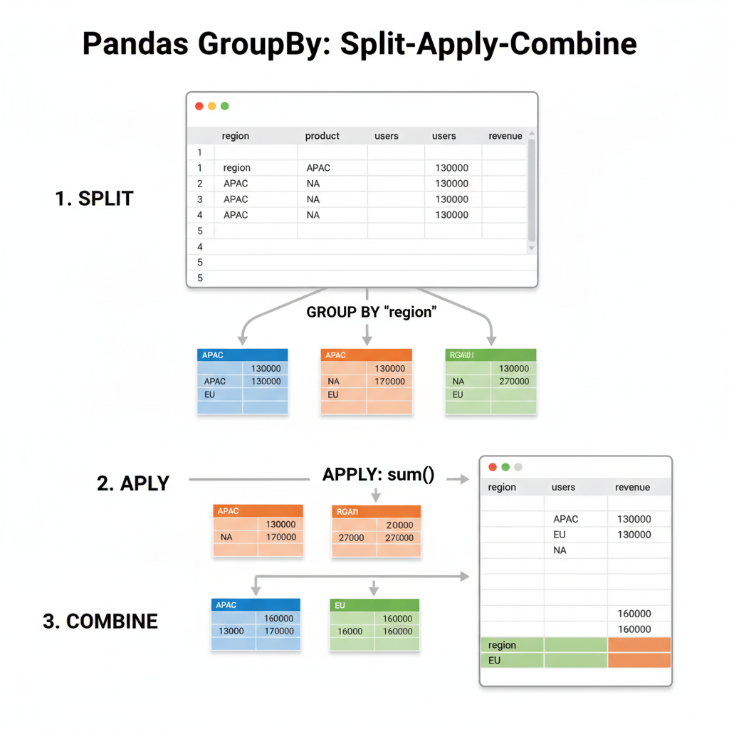 Sơ đồ: Visualization ba bước: (1) SPLIT - một DataFrame được chia thành các colored groups theo region (APAC=xanh dương, EU=xanh lá, NA=cam), (2) APPLY - mỗi group được apply sum() độc lập, (3) COMBINE - kết quả được merge lại thành một summary DataFrame. Dùng arrows để thể hiện flow.
# Custom aggregation với apply
def revenue_per_user(group):
    return pd.Series({
        'total_users': group['users'].sum(),
        'total_revenue': group['revenue'].sum(),
        'arpu': group['revenue'].sum() / group['users'].sum()
    })

usage.groupby('region').apply(revenue_per_user)
Merging DataFrames: Tương đương JOIN
Nếu bạn đã viết Room relations với @Embedded và @Relation, bạn sẽ thấy quen thuộc với pandas merge operations.
# Hai tables để join
users = pd.DataFrame({
    'user_id': [1, 2, 3, 4],
    'name': ['Alice', 'Bob', 'Charlie', 'Diana']
})

orders = pd.DataFrame({
    'order_id': [101, 102, 103, 104, 105],
    'user_id': [1, 2, 1, 3, 5],  # Lưu ý: user 5 không tồn tại trong users
    'amount': [50, 75, 30, 100, 25]
})

# Inner join (default) - chỉ matching records
merged = pd.merge(users, orders, on='user_id')
# user_id     name  order_id  amount
#       1    Alice       101      50
#       1    Alice       103      30
#       2      Bob       102      75
#       3  Charlie       104     100

# Left join - tất cả users, matched orders hoặc NaN
merged = pd.merge(users, orders, on='user_id', how='left')

# Outer join - tất cả records từ cả hai tables
merged = pd.merge(users, orders, on='user_id', how='outer')
Pandas how= | SQL Equivalent | Room Equivalent |
|---|---|---|
'inner' | INNER JOIN | @Relation với matching keys |
'left' | LEFT OUTER JOIN | @Relation với nullable result |
'right' | RIGHT OUTER JOIN | (ít phổ biến) |
'outer' | FULL OUTER JOIN | (implement thủ công) |
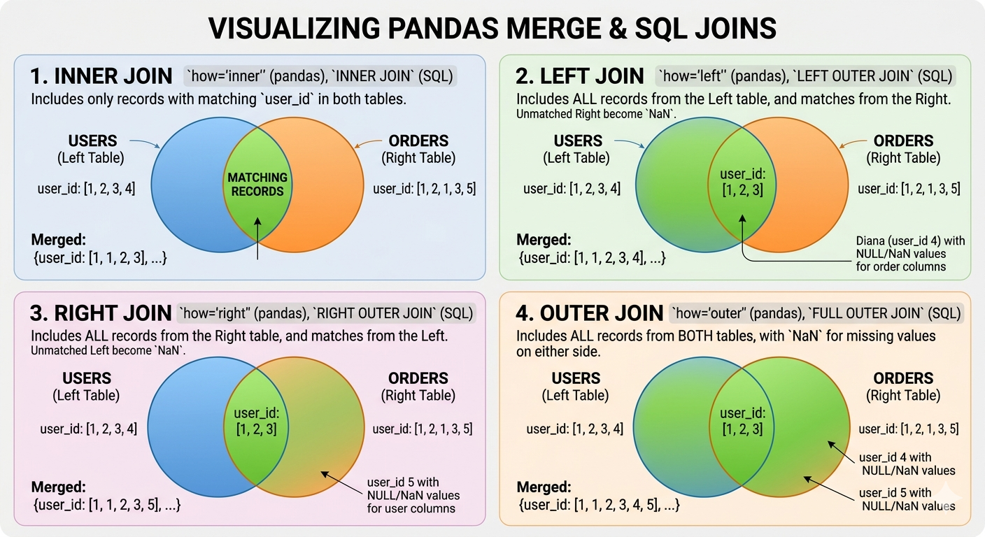 Sơ đồ: Bốn Venn diagram cho INNER (chỉ intersection), LEFT (tất cả left + matching right), RIGHT (tất cả right + matching left), và OUTER (union cả hai) joins. Dùng hai vòng tròn chồng nhau đại diện cho tables ‘users’ và ‘orders’, với colored regions thể hiện records nào được include trong mỗi loại join.
Method Chaining: Fluent API của Pandas
Một trong những thứ mình thích về Kotlin là method chaining với scope functions. Pandas có fluent API tương tự giúp data pipelines dễ đọc:
# Cách xấu (intermediate variables)
df1 = pd.read_csv('sales.csv')
df2 = df1.dropna()
df3 = df2[df2['region'] == 'APAC']
df4 = df3.groupby('product').sum()
result = df4.sort_values('revenue', ascending=False)

# Cách pandas (method chaining)
result = (pd.read_csv('sales.csv')
          .dropna()
          .query('region == "APAC"')
          .groupby('product')
          .sum()
          .sort_values('revenue', ascending=False))
Dấu ngoặc cho phép xuống dòng mà không cần backslashes. Đọc gần như một SQL query hoặc Kotlin Flow chain.
Method .pipe() cho Custom Functions
Khi bạn cần chèn custom logic vào một chain:
def add_revenue_category(df):
    df['category'] = pd.cut(df['revenue'],
                           bins=[0, 1000, 10000, float('inf')],
                           labels=['Small', 'Medium', 'Large'])
    return df

result = (pd.read_csv('sales.csv')
          .dropna()
          .pipe(add_revenue_category)  # Custom function trong chain
          .groupby('category')
          .sum())
Giống như Kotlin’s .let{} — cho phép bạn inject arbitrary transformations vào một fluent chain.
Cân nhắc về Performance
Quy tắc Vectorization vẫn áp dụng
Mọi thứ chúng ta học về NumPy vectorization đều áp dụng cho pandas:
import numpy as np

# CHẬM: iterate qua rows
def slow_calculate(df):
    results = []
    for idx, row in df.iterrows():
        results.append(row['a'] * 2 + row['b'])
    return results

# NHANH: vectorized operation
def fast_calculate(df):
    return df['a'] * 2 + df['b']
Benchmark trên 1 triệu rows:
- Version
iterrows(): ~45 giây - Version vectorized: ~15 milliseconds
Đó là speedup 3000 lần. Đừng bao giờ dùng iterrows() cho computation.
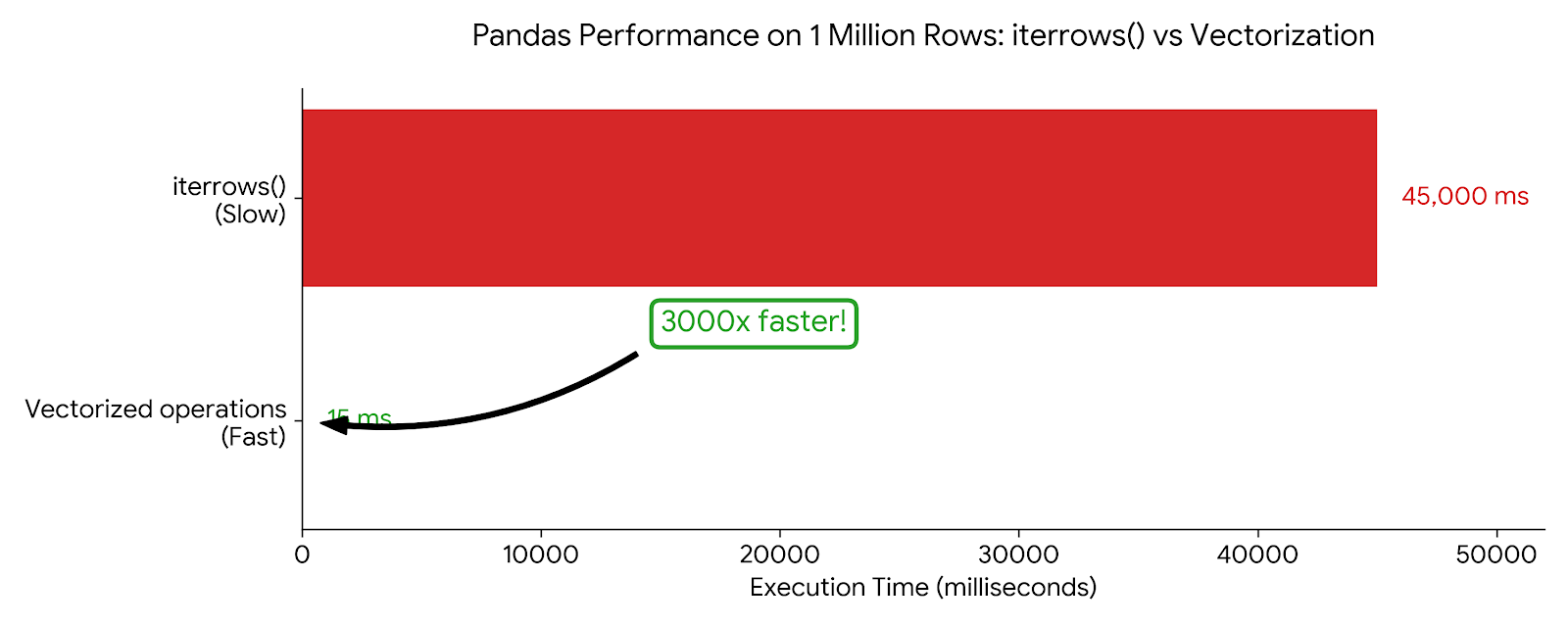 Biểu đồ: Horizontal bar chart so sánh iterrows() (45,000ms, đỏ/chậm) với vectorized operations (15ms, xanh/nhanh) trên 1 triệu rows. Bao gồm callout “3000x faster”. Tỷ lệ visual phải cho thấy sự khác biệt dramatic.
Memory Efficiency với dtypes
Pandas infer dtypes khi đọc data, nhưng thường lãng phí:
df = pd.read_csv('users.csv')
df.dtypes
# user_id      int64     # 8 bytes mỗi value
# age          int64     # 8 bytes, nhưng ages fit trong int8!
# is_premium   object    # Python objects, rất expensive

# Optimize
df['age'] = df['age'].astype('int8')           # 1 byte
df['is_premium'] = df['is_premium'].astype('bool')  # 1 byte (trước đó ~50+ bytes)
df['user_id'] = df['user_id'].astype('int32')  # 4 bytes

# Hoặc specify dtypes khi read
df = pd.read_csv('users.csv', dtype={
    'user_id': 'int32',
    'age': 'int8',
    'is_premium': 'bool'
})
Giống như việc chọn đúng data types trong Android để minimize APK size và memory footprint.
Category dtype cho Strings
Nếu một string column có repeated values (như regions, categories, status), dùng category:
# Trước: mỗi 'APAC' string được lưu riêng
df['region'].memory_usage(deep=True)  # 800000 bytes

# Sau: integers với lookup table
df['region'] = df['region'].astype('category')
df['region'].memory_usage(deep=True)  # 100300 bytes (giảm 88%!)
Chính xác như Android’s string resources — lưu một lần, reference nhiều lần.
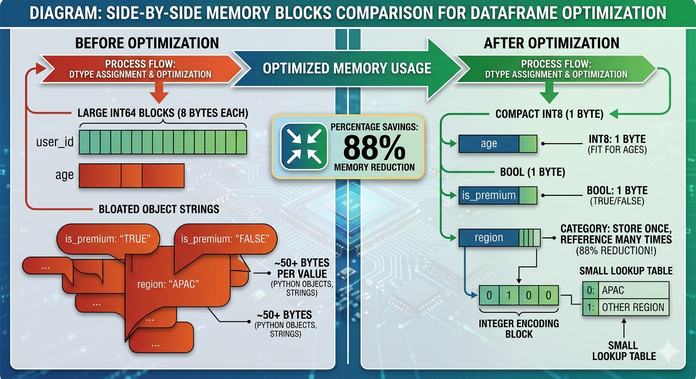 Sơ đồ: So sánh memory blocks cạnh nhau. Bên trái cho thấy “Before optimization” với các blocks int64 lớn (8 bytes mỗi cái) và object strings cồng kềnh. Bên phải cho thấy “After optimization” với int8 compact (1 byte), bool (1 byte), và category dtype (integer + small lookup table). Bao gồm percentage savings: “88% memory reduction”.
Các cạm bẫy thường gặp
1. SettingWithCopyWarning
Đây là error confusing nhất cho người mới học pandas:
# Cái này có thể work, nhưng là view hay copy?
subset = df[df['score'] > 80]
subset['grade'] = 'A'  # SettingWithCopyWarning!
Vấn đề: df[df['score'] > 80] có thể return một view (shared memory) hoặc một copy (independent memory). Modify nó có thể affect original df… hoặc không.
Cách fix: Be explicit về copies:
# Explicit copy
subset = df[df['score'] > 80].copy()
subset['grade'] = 'A'  # Safe, không warning

# Hoặc dùng .loc để in-place modification của original
df.loc[df['score'] > 80, 'grade'] = 'A'  # Modifies df trực tiếp
2. Chained Indexing là evil
# XẤU: chained indexing (không đoán được)
df['score'][0] = 100

# TỐT: single .loc call
df.loc[0, 'score'] = 100
3. “Feature” Index Alignment
Khi operate trên hai Series, pandas align theo index, không phải position:
s1 = pd.Series([1, 2, 3], index=['a', 'b', 'c'])
s2 = pd.Series([10, 20, 30], index=['b', 'c', 'd'])

s1 + s2
# a     NaN  # Không có 'a' trong s2
# b    12.0  # 2 + 10
# c    23.0  # 3 + 20
# d     NaN  # Không có 'd' trong s1
Điều này powerful cho time series data, nhưng surprising nếu bạn expect position-based operations. Dùng .values để lấy raw NumPy arrays nếu bạn cần position-based math.
Ví dụ thực tế: Phân tích dữ liệu App Store
Hãy kết hợp tất cả với một ví dụ realistic — phân tích app download data:
import pandas as pd
import numpy as np

# Load data
df = pd.read_csv('app_downloads.csv')

# Initial exploration
print(df.shape)           # (rows, columns)
print(df.dtypes)          # Column types
print(df.describe())      # Statistical summary
print(df.isna().sum())    # Missing values mỗi column

# Clean the data
df_clean = (df
    .dropna(subset=['revenue', 'downloads'])  # Required fields
    .fillna({'rating': df['rating'].median()})  # Fill optional với median
    .query('downloads > 0')  # Remove invalid records
)

# Feature engineering
df_clean['revenue_per_download'] = df_clean['revenue'] / df_clean['downloads']
df_clean['is_high_rated'] = df_clean['rating'] >= 4.5

# Analyze theo category
summary = (df_clean
    .groupby('category')
    .agg({
        'downloads': ['sum', 'mean'],
        'revenue': ['sum', 'mean'],
        'revenue_per_download': 'mean',
        'is_high_rated': 'mean'  # Tỷ lệ high-rated apps
    })
    .round(2)
    .sort_values(('revenue', 'sum'), ascending=False)
)

print(summary)
Đây là loại analysis mà trong Java sẽ cần hàng trăm dòng code, với manual null checks, loops, và temporary collections. Pandas làm trong vài dòng dễ đọc.
Tiếp theo
Chúng ta đã cover core của pandas — đủ để bắt đầu làm real data analysis. Trong bài tiếp theo, chúng ta sẽ tackle data visualization với matplotlib và seaborn — biến các DataFrames này thành charts kể chuyện.
Nhưng bài test thực sự đến khi bạn apply các tools này vào messy, real-world data. Kaggle dataset trông clean trong preview? Nó có Unicode issues, mixed date formats, và columns lẽ ra là numbers nhưng được lưu dưới dạng strings với commas.
Đó là nơi 80% công việc data science xảy ra. Và giờ bạn đã có tools để handle nó.
Key Takeaways
- DataFrame = Table: Nghĩ nó như dictionary của Series (columns) với shared index
- Vectorize mọi thứ: Đừng bao giờ dùng
iterrows()cho computation .loc[]cho labels,.iloc[]cho positions: Nhớ sự khác biệt inclusive vs exclusive slicing- Method chaining: Viết pipelines, không phải intermediate variables
- Be explicit về copies: Dùng
.copy()để tránh SettingWithCopyWarning - Optimize dtypes: Dùng
categorycho repeated strings, smaller ints cho bounded values
Với Android developers, sự thay đổi mental model tương tự như đi từ imperative Java sang declarative Kotlin Flow hoặc Compose. Bạn describe what bạn muốn, không phải how để compute từng bước.
Hẹn gặp ở bài tiếp theo!
Happy learning!